|
|
|
|
|
|
|
|
|
|
| Hybrid Model and Analysis, part 2
|
|
| Linear Model | |
| Figure 32 Sample disturbed trajectory (lo_hipK) |
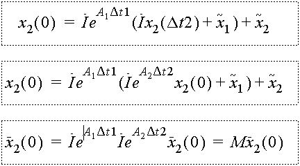
Assume that the dynamics within each mode is governed by linear equations, given by the matrices Ai. Given the reset dynamics in the last section, the return map from x2(0) to the next x2(0) is given by:
The last equation relates deviations, or disturbances, from the nominal trajectory. Interestingly, the existence of an periodic orbit does not depend on both modes being stable. However, in order for the orbit to be an attracting orbit, the eigenvalues of M must be inside the unit circle. |
| Safe Set | |
| Figure 33 Map of velocity disturbances to Safe Boundary (lo_hipK) Figure 34 In the above figures, the maximum velocity disturbances are shown in magenta, while the end states are shown in green. |
Even though the above equations show that a linear model of the system can be globally stable, in practice we cannot expect the system to recover from large perturbations. Foot slippage, breaking ground contact, and other unmodeled effects limit the robustness of even such a simplified system.
We define the safe set as the set of positions of the center of mass inside the "triangle of support", which is the geometric triangle formed by the three footholds of a given tripod. Although moving outside this set does not necessarily imply failure (the cockroach has been known to move outside this triangle during fast running), it does represent zones in which our stability can be compromised. In this formulation of the hybrid model, disturbances in position do not make sense, since they are ignored at the mode switch. Therefore, the question is: what range of velocity disturbances to the initial condition of a mode will result in the center of mass leaving the triangle of support? This problem is simplified given the fact that we know the length of time that the system is in that mode. Given the set of points that represent the boundary of the triangle of support, the above linear system can solved for the set of disturbances that will achieve this. However, for the full non-linear system, we resolve to simple numerical search. Our first assumption is to ignore disturbances in the rotational velocity, we only consider X and Y velocity disturbances. The second assumption is that if a velocity disturbance in a particular direction will put the system at the boundary after dt seconds, then that is the maximum velocity disturbance in that direction. We assume that a smaller velocity will keep us inside the boundary and a large one will push us out of it. To find the approximate maximum velocity disturbances, I used the following algorithm:
Figure 33 and 34 show the mapping from the maximum disturbance velocities to the end positions at the boundary. |
