|
|
|
|
|
|
|
|
|
|
| Hybrid Model and Analysis, part 1
|
|
 |
These two sections describe a more formal definition of the horizontal-plane locomotion model as a hybrid, or discrete-continuous, system. Of particular interest is the assumption that mode switches are induced by a timer, or clock-driven input, and its implication for self-stabilizing behavior. We begin by hypothesizing the basic stabilizing mechanism from simulation results and then define the hybrid automata based on this mechanism. Linear approximations to this automata show that it can reject disturbances in a global sense. However, since this is generally not true for actual locomoting systems, we define a more realistic "safe" region and numerically find a set of disturbances that will result in trajectories into the "unsafe" region. |
| Stabilizing Mechanism | |
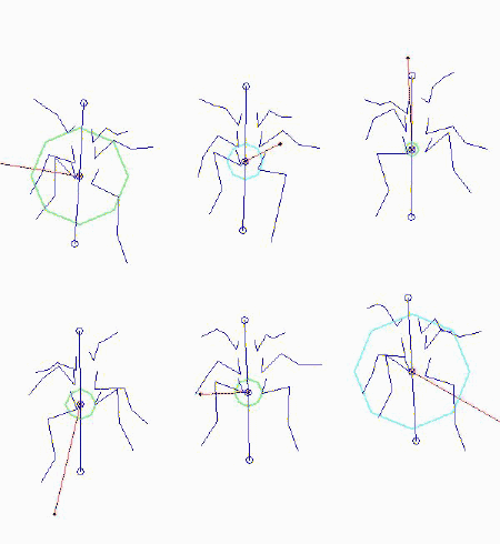
| Figure 25 Static Force-field for lo_hipK solution Figure 26 |
As seen in the previous section, simulations of the model produce self-stabilizing cyclic motion. By "self-stabilizing" I mean that the direction and speed of locomotion converge to finite values, despite disturbances in the system (see Figures 13 and 14).
In this document, I hypothesize that this behavior is the result of placing the state of the system away from a stable equilibrium at the start of the mode. The system then moves towards this equilibrium until it is time to switch into the next mode. The repeated "moving" of this equilibrium point results in motion of the system in a cyclic orbit. The stability of this equilibrium point results in the rejection of deviations from this nominal orbit. In this model there are two modes, one for each tripod of legs (please see the "Model" section for a description of the dynamics of the model; see the "Simulations" section for simulation movies). Figures 25 and 26 show the static force vector field for one of the modes. The "force-fields" were computed by fixing the footholds and then computing the resultant force exerted by the springs. This is the "static" force-field, since the effects of the viscous dampers are neglected. The resulting moments are represented by the circles, where the moment is proportional to the radius of the circle and the sign is represented by its color. As seen in the figures, there appears to be a static equilibrium point slightly above the front of the body for both sets of optimized parameters (please see "Optimization" section for a description of these two solutions). Note that the equilibrium point lies on different sides of the tripod in each model. The static force-fields points towards the equililbrium point almost uniformly, thereby motivating the above hypothesis. |
| Force field Comparison | |
| Figure 27 Forces along kinematic data trajectory Figure 28 Figure 29 |
Of course, it is difficult to compare the two force-fields of the models with the actual force-field of the animal, especially since we're only dealing with kinematic data.
Figures 27 shows the forces and moments along the trajectory of the kinematic data, estimated from the accelerations. Figures 28 and 29 show the forces along the trajectory for the two simulations. As shown, the pattern of forces in the animal more closely resembles the pattern in the hi_hipK simulations. |
| Model Definition | |
| Figure 30 Movie of simulated trajectory (lo_hipK) Figure 31 |
Motivated by the appearance of this equilibrium point, a convenient reference frame on which to define the model is this point. Since the leg footholds, and thus the equilibrium point, are determined with respect to the body regardless of orientation, this choice of frame conveniently allows us to always reset the position state of the body in the same place.
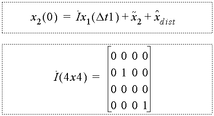
The hybrid model is defined as follows:
|
